Assembling data

• Sequence quality control (quality/adapter trimming, host decontamination)

• Assembly/co-assembly

• Evaluating an assembly

• Submitting primary assemblies to the ENA

Prerequisites

This tutorial requires Bandage which can be installed as per the github instructions for your system https://github.com/rrwick/Bandage#pre-built-binaries

For this tutorial you will need to make a working directory to store your data in:

mkdir -p ~/BiATA/session1/data
chmod -R 777 ~/BiATA
export DATADIR=~/BiATA/session1/data/session1

In this directory, download the tarball from http://ftp.ebi.ac.uk/pub/databases/metagenomics/mgnify_courses/biata_2021/

cd  ~/BiATA/session1/data/
wget -q http://ftp.ebi.ac.uk/pub/databases/metagenomics/mgnify_courses/biata_2021/session1.tgz
tar -xzvf session1.tgz

Now makes sure that you have pulled the docker container

docker pull microbiomeinformatics/biata-qc-assembly:v2021

Finally, start the docker container in the following way:

xhost +
docker run --rm -it  -e DISPLAY=$DISPLAY  -v $DATADIR:/opt/data -v /tmp/.X11-unix:/tmp/.X11-unix:rw -e DISPLAY=unix$DISPLAY microbiomeinformatics/biata-qc-assembly:v2021

Note that if running Docker windows, WSL must be disabled by selecting “Turn Windows features or or off” when Docker starts.

Part 1 - Quality control and filtering of the raw sequence files

 Learning Objectives - in the following exercises you will learn how to assess the quality of short read sequences, identify the presence of adapter sequences, and remove both adapters and low quality sequences. You will also learn how to construct a reference database for decontamination.

First go to your working area. The data that you downloaded has been mounted in /opt/data in the docker container.

cd /opt/data
ls

Here you should see the same contents as you had from downloading and uncompressing the session data. As we write into this directory, we should be able to see this from inside the container, and on the filesystem of the computer running this container. We will use this to our advantage as we go through this practical. Unless stated otherwise, all of the following commands should be executed in the terminal running the Docker container.

Generate a directory of the fastqc results

cd /opt/data
mkdir fastqc_results
cd fastqc_results
fastqc ../oral_human_example_1_splitaa.fastq.gz
fastqc ../oral_human_example_2_splitaa.fastq.gz
mv ../*html .
mv ../*zip .

Now on your local computer, go to the browser, and File -> Open File. Use the file navigator to select the following file

~/BiATA/session1/data/fastqc_results/oral_human_example_1_splitaa_fastqc.html

Spend some time looking at the ‘Per base sequence quality’.

For each position a BoxWhisker type plot is drawn. The elements of the plot are as follows:

• The central red line is the median value

• The yellow box represents the inter-quartile range (25-75%)

• The upper and lower whiskers represent the 10% and 90% points

• The blue line represents the mean quality

The y-axis on the graph shows the quality scores. The higher the score the better the base call. The background of the graph divides the y axis into very good quality calls (green), calls of reasonable quality (orange), and calls of poor quality (red). The quality of calls on most platforms will degrade as the run progresses, so it is common to see base calls falling into the orange area towards the end of a read.

What does this tell you about your sequence data? Where do the errors start?

In the pre-processed files we see two warnings, as shown on the left side of the report. Navigate to the “Per bases sequence content”

 At around 15-19 nucleotides, the DNA composition becomes very even but at the 5’ end of the sequence there  are distinct differences. Why do you think that is?

 Open up the FastQC report corresponding to the reversed reads.

Are there any significant differences between the forward and reverse reads?

For more information on the FastQC report, please consult the ‘Documentation’ available from this site: https://www.bioinformatics.babraham.ac.uk/projects/fastqc/

 We are currently only looking at two files but often we want to look at many files. The tool multiqc aggregates the FastQC results across many samples and creates a single report for easy comparison. Here we will demonstrate the use of this tool

cd /opt/data
mkdir multiqc_results
multiqc fastqc_results -o multiqc_results

In this case, we provide the folder containing the fastqc results to multiqc and the -o allows us to set the output directory for this summarised report.

Now on your local computer, open the summary report from MultiQC. To do so, go to your browser, and use File -> Open File. Use the file navigator to select the following file

~/BiATA/session1/data//multiqc_results/multiqc_report.html

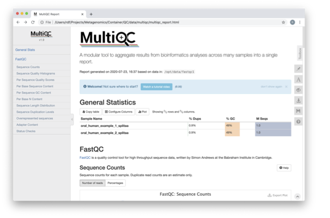
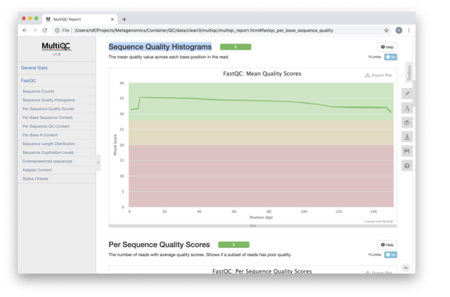
Scroll down through the report. The sequence quality histograms show the following results from each file as two separate lines. The ‘Status Checks’ show a matrix of which samples passed check and which ones have problems.

 What fraction of reads are duplicates?

So, far we have looked at the raw files and assessed their content, but we have not done anything about removing sequences with low quality scores or adapters. So, lets start this process. The first step in the process is to make a database relevant for decontaminating the sample. It is always good to routinely screen for human DNA (which may come from the host and/or staff performing the experiment). However, if the sample is say from mouse, you would want to download the the mouse genome instead.

In the following exercise, we are going to use two “genomes” already downloaded for you in the decontamination folder. To make this tutorial quicker and smaller in terms of file sizes, we are going to use PhiX (a common spike in) and just chromosome 10 from human.

cd /opt/data/decontamination

For the next step we need one file, so we want to merge the two different fasta files. This is simply done using the command line tool cat.

cat phix.fasta GRCh38_chr10.fasta > GRCh38_phix.fasta

Now we need to build a bowtie index for them:

bowtie2-build GRCh38_phix.fasta GRCh38_phix.index

It is possible to automatically download a pre-indexed human genome in Bowtie2 format using the following command (but do not do this now, as this will take a while to download):

kneaddata_database –download human_genome bowtie2

Now we are going to use the GRCh38_phix database and clean-up our raw sequences. kneaddata is a helpful wrapper script for a number of pre-processing tools, including Bowtie2 to screen out contaminant sequences, and Trimmomatic to exclude low-quality sequences. We also have written wrapper scripts to run these tools (see below), but using kneaddata allows for more flexibility in options.

cd /opt/data/
mkdir clean

We now need to uncompress the fastq files.

gunzip -c oral_human_example_2_splitaa.fastq.gz > oral_human_example_2_splitaa.fastq
gunzip -c oral_human_example_1_splitaa.fastq.gz > oral_human_example_1_splitaa.fastq

kneaddata --remove-intermediate-output -t 2 --input oral_human_example_1_splitaa.fastq --input oral_human_example_2_splitaa.fastq --output /opt/data/clean --reference-db /opt/data/decontamination/GRCh38_phix.index --trimmomatic-options  "SLIDINGWINDOW:4:20 MINLEN:50" --bowtie2-options "--very-sensitive --dovetail" --remove-intermediate-output

 The options above are:

* –input, Input FASTQ file. This option is given twice as we have paired-end data. * –output, Output directory. * –reference-db, Path to bowtie2 database for decontamination. * -t, # Number of threads to use (2 in this case). * –trimmomatic-options, Options for Trimmomatic to use, in quotations (“SLIDINGWINDOW:4:20 MINLEN:50” in this case). See the Trimmomatic website for more options. * –bowtie2-options, Options for bowtie2 to use, in quotations. The options “–very-sensitive” and “–dovetail” set the alignment parameters to be very sensitive and sets cases where mates extend past each other to be concordant (i.e. they will be called as contaminants and be excluded). * –remove-intermediate-output, Intermediate files, including large FASTQs, will be removed.

Kneaddata generates multiple outputs in the “clean” directory, containing different 4 different files for each read.

 Using what you have learned previously, generate a fastqc report for each of the oral_human_example_1_splitaa_kneaddata_paired files.  Do this within the clean directory.

cd /opt/data/clean
mkdir fastqc_final
<you construct the command>

Also generate a multiqc report and look at the sequence quality historgrams.

cd /opt/data/clean
mkdir multiqc
<you construct the command>

View the multiQC report as before using your browser. You should see something like this:

Open the previous MultiQC report and see have they have improved?

Did sequences at the 5’ end become uniform? Why might that be? Is there anything that suggests that adapter sequences were found?

To generate a summary file of how the sequence were categorised by Kneaddata, run the following command.

cd /opt/data
kneaddata_read_count_table --input /opt/data/clean --output kneaddata_read_counts.txt
less kneaddata_read_counts.txt

What fraction of reads were deemed to be contaminating?

 The reads have now be decontaminated any can be uploaded to ENA, one of the INSDC members. It is beyond the scope of this course to include a tutorial on how to submit to ENA, but there is additional information available on how to do this in this Online Training guide provided by EMBL-EBI

https://www.ebi.ac.uk/training/online/course/ebi-metagenomics-portal-submitting-metagenomics-da/considerations-submitting-metagenomic-data

Part 2 - Assembly and Co-assembly

 Learning Objectives - in the following exercises you will learn how to perform a metagenomic assembly and to start some basic analysis of the output. Subsequently, we will demonstrate the application of co-assembly. Note, due to the complexity of metagenomics assembly, we will only be investigating very simple example datasets as these often take days of CPU time and 100s of GB of memory. Thus, do not think that there is an issue with the assemblies.

Once you have quality filtered your sequencing reads (see Part 1 of this session), you may want to perform de novo assembly in addition to, or as an alternative to a read-based analyses. The first step is to assemble your sequences into contigs. There are many tools available for this, such as MetaVelvet, metaSPAdes, IDBA-UD, MegaHIT. We generally use metaSPAdes, as in most cases it yields the best contig size statistics (i.e. more continguous assembly) and has been shown to be able to capture high degrees of community diversity (Vollmers, et al. PLOS One 2017). However, you should consider the pros and cons of different assemblers, which not only includes the accuracy of the assembly, but also their computational overhead. Compare these factors to what you have available. For example, very diverse samples with a lot of sequence data uses a lot of memory with SPAdes. In the following practicals we will demonstrate the use of metaSPAdes on a small sample and the use of MegaHIT for performing co-assembly.

 Using the sequences that you have previously QC-ed, run metaspades. To make things faster, we are going to turn-off metaspades own read error correction method, by specifying the command –only-assembler.

cd /opt/data
mkdir assembly
metaspades.py \
        -t 2  \
        --only-assembler \
        -m 10 \
        -1 /opt/data/clean/oral_human_example_1_splitaa_kneaddata_paired_1.fastq \
        -2 /opt/data/clean/oral_human_example_1_splitaa_kneaddata_paired_2.fastq \
        -o /opt/data/assembly

 This takes about 1 hour to complete.

 Once this completes, we can investigate the assembly. The first step is to simply look at the contigs.fasta file.

Now take the first 40 lines of the sequence and perform a blast search at NCBI (https://blast.ncbi.nlm.nih.gov/Blast.cgi, choose Nucleotide:Nucleotide from the set of options). Leave all other options as default on the search page. To select the first 40 lines of sequence perform the following:

head -41 contigs.fasta

 Which species do you think this sequence may be coming from? Does this make sense as a human oral bacteria? Are you surprised by this result at all?

Now let us consider some statistics about the entire assembly

cd /opt/data/assembly
assembly_stats scaffolds.fasta

 This will output two simple tables in JSON format, but it is fairly simple to read. There is a section that corresponds to the scaffolds in the assembly and a section that corresponds to the contigs.

 What is the length of longest and shortest contigs?

 What is the N50 of the assembly? Given that are input sequences were ~150bp long paired-end sequences, what does this tell you about the assembly?

 N50 is a measure to describe the quality of assembled genomes that are fragmented in contigs of different length.  We can apply this with some caution to metagenomes, where we can use it to crudely assess the contig length that covers 50% of the total assembly.  Essentially the longer the better, but this only makes sense when thinking about alike metagenomes. Note, N10 is the minimum contig length to cover 10 percent of the metagenome. N90 is the minimum contig length to cover 90 percent of the metagenome.

 In addition to evaluating the contiguity the assemblies, we can ask what fraction of the diversity in the samples was assembled. We can answer this question by quantifying the number of reads that map to the assembly. BWA expects that the read names in the forward and reverse reads are the same so we will first remove the read identifiers and make sure that they are ordered correctly.

sed 's/\/1//g' ../clean/oral_human_example_1_splitaa_kneaddata_paired_1.fastq > ../clean/oral_human_example_1_splitaa_kneaddata_paired_noidentifiers_1.fastq
sed 's/\/2//g' ../clean/oral_human_example_1_splitaa_kneaddata_paired_2.fastq > ../clean/oral_human_example_1_splitaa_kneaddata_paired_noidentifiers_2.fastq
repair.sh in=../clean/oral_human_example_1_splitaa_kneaddata_paired_noidentifiers_1.fastq in2=../clean/oral_human_example_1_splitaa_kneaddata_paired_noidentifiers_2.fastq out=../clean/oral_human_example_1_splitaa_kneaddata_paired_noidordered_1.fastq out2=../clean/oral_human_example_1_splitaa_kneaddata_paired_noidordered_2.fastq

To calculate the percent reads mapping to the assembly using the flagstat output generated in the previous step, calculate the number of primary alignments (mapped - secondary - supplementary). Then divide the number of primary alignments by the sum of forward and reverse reads to get the fraction of reads mapped.

bwa index scaffolds.fasta
bwa mem -t 2 scaffolds.fasta ../clean/oral_human_example_1_splitaa_kneaddata_paired_noidordered_1.fastq ../clean/oral_human_example_1_splitaa_kneaddata_paired_noidordered_2.fastq | samtools view -bS - | samtools sort -@ 2 -o oral_human_example_1_splitaa.sam -
samtools flagstat oral_human_example_1_splitaa.sam > oral_human_example_1_splitaa_flagstat.txt

To get the total number of reads in the forward read, run the command below and divide by 4. Repeat for the reverse read.

wc -l ../clean/oral_human_example_1_splitaa_kneaddata_paired_noidordered_1.fastq
wc -l ../clean/oral_human_example_1_splitaa_kneaddata_paired_noidordered_2.fastq

 What percent of the reads were incorporated into the assembly? What factors can affect the percent of reads mapping to the assembly?

 Bandage (a Bioinformatics Application for Navigating De novo Assembly Graphs Easily), is a program that creates interactive visualisations of assembly graphs. They can be useful for finding sections of the graph, such as rRNA, or to try to find parts of a genome. Note, you can install Bandage on your local system - see the prerequisites section. With Bandage, you can zoom and pan around the graph and search for sequences, plus much more. The following guide allows you to look at the assembly graph.  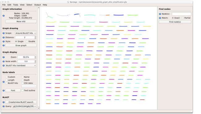Normally, I would recommend looking at the ‘ assembly_graph.fastg, but our assembly is quite fragmented, so we will load up the assembly_graph_after_simplification.gfa.

Open Bandage

In the the Bandage GUI perform the following

Select File->Load graph

Navigate to  ~/BiATA/session1/data/session1/assembly and select on assembly_graph_after_simplification.gfa

Once loaded, you need to draw the graph. To do so, under the “Graph drawing” panel on the left side perform the following:

Set Scope to ‘Entire graph’

The click on Draw graph

 Use the sliders in the main panel to move around and look at each distinct part of the assembly graph.

 Can you find any large, complex parts of the graph? If so, what do they look like.

In this particular sample, we believe that strains related to the species Rothia dentocariosa, a Gram-positive, round- to rod-shaped bacteria that is part of the normal community of microbes residing in the mouth and respiratory tract, should be present in our sample. While this is a tiny dataset, lets try to see if there is evidence for this genome. To do so, we will search the R. dentocariosa genome against the assembly graph.

To do so, go to the “BLAST” panel on the left side of the GUI.

Step 1 - Select Create/view BLAST search, this will open a new window

Step 2 - select build Blast database

Step 3 - Load from FASTA file -> navigate to the genome folder /opt/data/genome and select GCA_000164695.fasta

Step 4 - modify the  blast filters to 95% identity

Step 6 - run blast

Step 7 - close this window

To visualise just these hits, go back to “Graph drawing” panel.

Set Scope to ‘Around BLAST hits’

Set Distance 2

The click on Draw graph

You should then see something like this:

 In the following steps of this exercise, we will look at performing co-assembly of multiple datasets. Due to computational limitations, we can only look a example datasets.  However, the principles are the same. We have also pre-calculated some assemblies for you. In the co-assembly directory, there are already 2 assemblies.  We have a single paired-end assembly.

megahit -1 clean_other/oral_human_example_1_splitac_kneaddata_paired_1.fastq -2 clean_other/oral_human_example_1_splitac_kneaddata_paired_1.fastq -o coassembly/assembly1 -t 2 --k-list 23,51,77

Now run the assembly_stats on the contigs for this assembly.

cd /opt/data
assembly_stats coassembly/assembly1/final.contigs.fa

How do these differ to the ones you generated previously? What may account for these differences?

 We have also generated the first coassembly using MegaHIT. This was produced using the following command.  To specify the files, we put all of the forward file as a comma separated list, and all of the reversed as a comma separated list, which should be ordered that same in both, such that the mate pairs match up.

cd /opt/data
megahit -1 clean_other/oral_human_example_1_splitac_kneaddata_paired_1.fastq,clean_other/oral_human_example_1_splitab_kneaddata_paired_1.fastq -2 clean_other/oral_human_example_1_splitac_kneaddata_paired_1.fastq,clean_other/oral_human_example_1_splitab_kneaddata_paired_2.fastq -o coassembly/assembly2 -t 2 --k-list 23,51,77

Now perform another co-assembly:

megahit -1 clean_other/oral_human_example_1_splitab_kneaddata_paired_1.fastq,clean_other/oral_human_example_1_splitac_kneaddata_paired_1.fastq,clean/oral_human_example_1_splitaa_kneaddata_paired_1.fastq -2 clean_other/oral_human_example_1_splitab_kneaddata_paired_2.fastq,clean_other/oral_human_example_1_splitac_kneaddata_paired_2.fastq,clean/oral_human_example_1_splitaa_kneaddata_paired_2.fastq -o coassembly/assembly3 -t 2 --k-list 23,51,77

 This takes about 20-30 minutes. Also, if you are using a laptop, make sure that it does not go into standby mode.

 You should now have three different assemblies, two provide and one generated by yourselves. Now let us compare the assemblies.

cd /opt/data
assembly_stats coassembly/assembly1/final.contigs.fa
assembly_stats coassembly/assembly2/final.contigs.fa
assembly_stats coassembly/assembly3/final.contigs.fa

 We only have contigs.fa from MegaHIT, so the contigs and scaffold sections are the same.

Has the assembly improved? If so how?