Viral detection and classification
Prerequisites
IMPORTANT: It is strongly recommended that you complete section 1.1 below (setting up the computing environment) prior to the practical session. Depending on your available network it can take some time (1-2 hrs) to download the necessary files.
 1.1. To run this tutorial first we need to set up our computing environment in order to execute the commands as listed here. First, download and the virify_tutorial.tar.gz file containing all the data you will need using any of the following options:
wget http://ftp.ebi.ac.uk/pub/databases/metagenomics/mgnify_courses/biata_2021/virify_tutorial.tar.gz
or
rsync -av --partial --progress rsync://ftp.ebi.ac.uk/pub/databases/metagenomics/mgnify_courses/biata_2021/virify_tutorial.tar.gz .
Once downloaded, extract the files from the tarball:
tar -xzvf virify_tutorial.tar.gz
Now change into the virify_tutorial directory and setup the environment by running the following commands in your current terminal session:
cd virify_tutorial
docker load --input docker/virify.tar
docker run --rm -it -v $(pwd)/data:/opt/data virify
mkdir obs_results
All commands detailed below will be run from within this current working directory. Note: if there are any issues in running this tutorial, there is a separate directory exp_results/ with pre-computed results.
1. Identification of putative viral sequences
 In order to retrieve putative viral sequences from a set of metagenomic contigs we are going to use two different tools designed for this purpose, each of which employs a different strategy for viral sequence detection: VirFinder and VirSorter. VirFinder uses a prediction model based on kmer profiles trained using a reference database of viral and prokaryotic sequences. In contrast, VirSorter mainly relies on the comparison of predicted proteins with a comprehensive database of viral proteins and profile HMMs. The VIRify pipeline uses both tools as they provide complementary results:
VirFinder performs better than VirSorter for short contigs (<3kb) and includes a prediction model suitable for detecting both eukaryotic and prokaryotic viruses (phages).
In addition to reporting the presence of phage contigs, VirSorter detects and reports the presence of prophage sequences (phages integrated in contigs containing their prokaryotic hosts).
1.2 In the current working directory you will find the metagenomic assembly we will be working with (ERR575691_host_filtered.fasta). We will now filter the contigs listed in this file to keep only those that are ≥500 bp, by using the custom python script filter_contigs_len.py as follows:
filter_contigs_len.py -f ERR575691_host_filtered.fasta -l 0.5 -o obs_results/ERR575691_host_filtered_filt500bp.fasta
1.3. The output from this command is a file named ERR575691_host_filtered_filt500bp.fasta which is located in the obs_results diretory. Our dataset is now ready to be processed for the detection of putative viral sequences. We will first analyse it with VirFinder using a custom R script:
VirFinder_analysis_Euk.R -f obs_results/ERR575691_host_filtered_filt500bp.fasta -o obs_results
1.4. Following the execution of the R script you will see a tabular file (obs_results/ERR575691_host_filtered_filt500bp_VirFinder_table-all.tab) that collates the results obtained for each contig from the processed FASTA file. The next step will be to analyse the metagenomic assembly using VirSorter. To do this run:
wrapper_phage_contigs_sorter_iPlant.pl -f obs_results/ERR575691_host_filtered_filt500bp.fasta --db 2 --wdir obs_results/virsorter_output --virome --data-dir /opt/data/databases/virsorter-data
VirSorter classifies its predictions into different confidence categories:
Category 1: “most confident” predictions
Category 2: “likely” predictions
Category 3: “possible” predictions
Categories 4-6: predicted prophages
1.5. While VirSorter is running, we have prepared an R script so you can inspect the VirFinder results in the meantime using ggplot2. Open RStudio and load the Analyse_VirFinder.R script located in the /virify_tutorial/data/scripts/ directory. Run the script (press Source on the top right corner) to generate the plot. (If you don’t have RStudio, or don’t care to run this you can just look at the resulting plot in the image below)
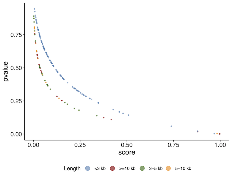
As you can see there is a relationship between the p-value and the score. A higher score or lower p-value indicates a higher likelihood of the sequence being a viral sequence. You will also notice that the results correlate with the contig length. The curves are slightly different depending on whether the contigs are > or < than 3kb. This is because VirFinder uses different machine learning models at these different levels of length.
1.6. Once VirSorter finishes running, we then generate the corresponding viral sequence FASTA files using a custom python script (parse_viral_pred.py) as follows:
parse_viral_pred.py -a obs_results/ERR575691_host_filtered_filt500bp.fasta -f obs_results/ERR575691_host_filtered_filt500bp_VirFinder_table-all.tab -s obs_results/virsorter_output -o obs_results
Following the execution of this command, FASTA files (*.fna) will be generated for each one of the VIRify categories mentioned above containing the corresponding putative viral sequences.
The VIRify pipeline takes the output from VirFinder and VirSorter, reporting three prediction categories:
High confidence: VirSorter phage predictions from categories 1 and 2.
Low confidence:
Contigs that VirFinder reported with p-value < 0.05 and score ≥ 0.9.
Contigs that VirFinder reported with p-value < 0.05 and score ≥ 0.7, but that are also reported by VirSorter in category 3.
Prophages: VirSorter prophage predictions categories 4 and 5.
2. Detection of viral taxonomic markers
Once we have retrieved the putative viral sequences from the metagenomic assembly, the following step will be to analyse the proteins encoded in them in order to identify any viral taxonomic markers. To carry out this identification, we will employ a database of profile Hidden Markov Models (HMMs) built from proteins encoded in viral reference genomes. These profile HMMs were selected as viral taxonomic markers following a comprehensive random forest-based analysis carried out previously.
2.1. The VIRify pipeline uses prodigal for the detection of protein coding sequences (CDSs) and hmmscan for the alignment of the encoded proteins to each of the profile HMMs stored in the aforementioned database. We will use the custom script Generate_vphmm_hmmer_matrix.py to conduct these steps for each one of the FASTA files sequentially in a “for loop”. In your terminal session, execute the following command:
for file in $(find obs_results/ -name '*.fna' -type f | grep -i 'putative'); do Generate_vphmm_hmmer_matrix.py -f ${file} -o ${file%/*}; done
Once the command execution finishes two new files will be stored for each category of viral predictions. The file with the suffix CDS.faa lists the proteins encoded in the CDSs reported by prodigal, whereas the file with the suffix hmmer_ViPhOG.tbl contains all significant alignments between the encoded proteins and the profile HMMs, on a per-domain-hit basis.
2.2. The following command is used to parse the hmmer output and generate a new tabular file that lists alignment results in a per-query basis, which include the alignment ratio and absolute value of total E-value for each protein-profile HMM pair.
for file in $(find obs_results/ -name '*ViPhOG.tbl' -type f); do Ratio_Evalue_table.py -i ${file} -o ${file%/*}; done
3. Viral taxonomic assignment
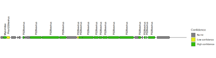
The final output of the VIRify pipeline includes a series of gene maps generated for each putative viral sequence and a tabular file that reports the taxonomic lineage assigned to each viral contig. The gene maps provide a convenient way of visualizing the taxonomic annotations obtained for each putative viral contig and compare the annotation results with the corresponding assigned taxonomic lineage. Taxonomic lineage assignment is carried out from the highest taxonomic rank (genus) to the lowest (order), taking all the corresponding annotations and assessing whether the most commonly reported one passes a pre-defined assignment threshold.
3.1. First, we are going to generate a tabular file that lists the taxonomic annotation results obtained for each protein from the putative viral contigs. We will generate this file for the putative viral sequences in each prediction category. Run the following:
for file in $(find obs_results/ -name '*CDS.faa' -type f); do viral_contigs_annotation.py -p ${file} -t ${file%CDS.faa}hmmer_ViPhOG_informative.tsv -o ${file%/*}; done
3.2. Next, we will take the tabular annotation files generated and use them to create the viral contig gene maps. To achieve this, run the following:
for file in $(find obs_results/ -name '*annot.tsv' -type f); do Make_viral_contig_map.R -t ${file} -o ${file%/*}; done
3.3. Finally, we will use the tabular annotation files again to carry out the taxonomic lineage assignment for each putative viral contig. Run the following command:
for file in $(find obs_results/ -name '*annot.tsv' -type f); do contig_taxonomic_assign.py -i ${file} -o ${file%/*}; done
Final output results are stored in the obs_results/ directory.
The gene maps are stored per contig in individual PDF files (suffix names of the contigs indicate their level of confidence and category class obtained from VirSorter). Each protein coding sequence in the contig maps (PDFs) is coloured and labeled as high confidence (E-value < 0.1), low confidence (E-value > 0.1) or no hit, based on the matches to the HMM profiles. Do not confuse this with the high confidence or low confidence prediction of VIRify for the whole contig.
Taxonomic annotation results per classification category are stored as text in the *_tax_assign.tsv files.
Let’s inspect the results. Do:
cat obs_results/*tax_assign.tsv
You should see a list of 9 contigs detected as viral and their taxonomic annotation in separate columns (partitioned by taxonomic rank). However, some do not have an annotation (e.g. NODE_4… and NODE_5…).
Open the gene map PDF files of the corresponding contigs to understand why some contigs were not assigned to a taxonomic lineage. You will see that for these cases, either there were not enough genes matching the HMMs, or there was disagreement in their assignment.